I Built a World Cup Predictor. Could It Pick Match Results Better Than Elo?

• Research app: Open the app (opens in a new tab) (the first start may take a few minutes)
• Code and reports: GitHub repository (opens in a new tab)

In short

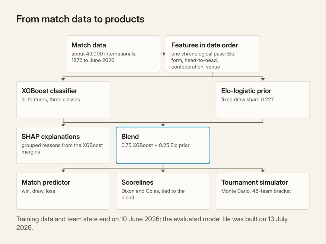
Can a machine-learning model forecast World Cup matches better than a plain Elo ratingElo ratingA strength score for each team, borrowed from chess. Every team starts at 1500; after each match, a team's rating changes by the gap between the actual result and the expected one, so even a draw can move it.See in the glossaryClose, a simple team-strength score? To find out, I built one for the 2026 FIFA World Cup: before each match it gives three probabilities, for a win, a draw and a loss. Behind it are an XGBoostXGBoostA machine-learning method that grows hundreds of small decision trees in sequence, each one correcting the mistakes of the trees before it.See in the glossaryClose model blended with Elo, a scoreline layer, plain-language explanations and a tournament simulator, all in a small public app. (The glossary at the end explains each term in a line.) Then I tested it twice: on three past World Cups (192 matches, with team state frozen on the eve of each tournament) and on all 104 matches of the 2026 World Cup, with training data that ends the day before the opening game.

Neither test produced a clean win. On the three past World Cups, Elo predicted more results correctly than my blend (56.25% against 53.1%), but the paired test found no statistically significant difference (p = 0.21p-valueIf the two systems were truly equally accurate, the probability of seeing a difference at least this large in the test. Here it comes from McNemar's test.See in the glossaryClose). At the 2026 World Cup, Elo again predicted two more results correctly (70 of 104 against 68), while the blendBlendThe model that combines, for each outcome, the XGBoost probability with weight 75% and the Elo prior with weight 25%. The app shows its probabilities.See in the glossaryClose's probabilities had a lower log-lossLog-lossA score for probability forecasts that rewards confident correct calls and punishes confident wrong ones. Lower is better.See in the glossaryClose, this time with a bootstrapPaired bootstrapResampling the same matches with replacement thousands of times, so that a match can appear more than once in a sample, and comparing both models on each resample to see how far the difference between their scores could swing. In this article it gives the intervals for the log-loss difference between the two models.See in the glossaryClose intervalConfidence intervalA range that shows the uncertainty of an estimate. Here, when the interval for the difference between two models includes zero, the data are also consistent with no difference.See in the glossaryClose that excludes zero. Only the last four forecasts were written down before kickoff; three came true, and Elo had picked the same four teams. The rest of this article explains why a near-tie with a simple baseline was the most informative result of the project, and what it says about predicting football from public match history.

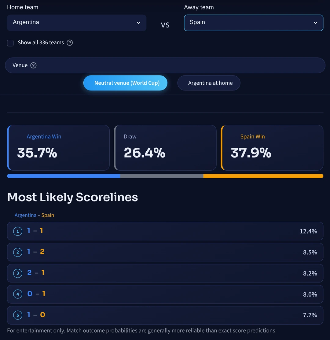
Why football is hard to predict

Football is hard to forecast, and the difficulty is structural. A match has three outcomes, and one of them, the draw, is the hardest to call: roughly a quarter of matches in the long English league record end level, and internationals draw at a similar or slightly lower rate. A large slice of every dataset lands in the one class hardest to call, which puts a ceiling on three-way accuracy.

Any football model also faces a demanding benchmark: the betting market. Forrest, Goddard and Simmons (2005) found that a sophisticated statistical model only matched, and did not consistently exceed, the bookmakers. So the question for a personal project is not "can I beat the market" but "can I build something well engineered and well calibrated, and learn where its limits are".

That is the question I set out to answer for the 2026 World Cup: the first 48-team edition, hosted across the United States, Canada and Mexico from 11 June to 19 July 2026, with 12 groups of four feeding a new 32-team knockout round.

The data, and what it does and does not tell you

The foundation is Mart Jürisoo's dataset International football results from 1872 to present (opens in a new tab): roughly 49,000 men's full international matches from the first official fixture in 1872 to the present, with date, teams, scores, tournament, venue and a neutral-venue flag. It excludes Olympic matches and B-team, under-23 and select-side fixtures, which is exactly what senior-international modelling wants.

Three caveats matter enough to state up front.

The target in knockouts. The dataset records full-time scores including extra time but excluding penalty shootouts. A match that is 1-1 after 90 minutes and 2-1 after extra time is stored as a decisive result, not a draw. So my win, draw and loss target is "the result after extra time, with shootouts treated as draws": closer to "who advances" than to the 90-minute market. That is reasonable for a tournament model, but it has to be stated, not assumed. The live tracker enforces the same convention and strips the shootout from the results feed, so a knockout decided on penalties is scored as the after-extra-time draw, exactly as in training.

The source keeps changing. The source repository updates continuously, including corrections to old matches, so a reproducible result needs a pinned snapshot. The processed history behind every number here is one frozen file of 49,404 matches ending on 10 June 2026, and its checksum, with the checksum of the trained model, is recorded in a manifest in the repository. A test fails if either file drifts. The cutoff date, the checksums and the source commit are listed in the details of the data snapshot used in this project (opens in a new tab).

Nothing from the future, with two disclosed exceptions. Every feature for a match is computed only from information available strictly before kickoff, and every backtest trains only on matches played before the tournament being evaluated. Two constants are the exceptions: the prior's draw share and the home-advantage shift are each fitted once on the whole history up to June 2026, so in the backtest they reflect matches played after the tournaments being tested. The feature and model sections below give the effect of each constant and the limits of how it was checked. This sounds obvious and is the single easiest thing to get quietly wrong; the evaluation section describes a place where my first evaluation got it subtly wrong anyway.

Feature engineering: an Elo backbone, built forward in time

The features are deliberately interpretable. The backbone is an Elo rating for every team. Elo, borrowed from chess (Elo, 1978), starts every team at 1500. After each match, each team's rating changes by the gap between the actual result and the expected one, so a draw against a much stronger team also earns points. The expected score for the home team is the standard logistic curve:

and after the match each rating moves by the surprise:

where S is 1, 0.5 or 0 for a home win, draw or loss. I use a constant K = 40, a pragmatic simplification rather than a tuned optimum. Production football Elo systems such as the World Football Elo Ratings vary K by match importance and goal margin; a constant K treats a friendly and a World Cup final as equally informative. I kept it constant because it is a transparent, strong baseline, and, as the results show, very hard to beat anyway.

On top of Elo, each match row carries recent form (win rate and average goal difference over the last 5 and 10 games, per team), head-to-head history (number of prior meetings and the first team's win rate in them), a confederation-strength feature (the average Elo of each team's confederation; in this data UEFA and CONMEBOL teams have higher average ratings than OFC teams), a neutral-venue flag and a World Cup flag. After one-hot encoding the confederations (one yes-or-no column per confederation), that is 31 features.

Crucially, all of this is built in one chronological walk through history: record the pre-match features, append the row, and only then update Elo, form and head-to-head state with the result. The features for each match therefore come only from matches played before it.

Venue. Most World Cup matches are on neutral ground, but a host nation plays at home. The system models this with one explicit contract: a neutral match is scored symmetrically (both team orderings averaged), and a host's match gives the host a fixed home-advantage shift of 125.58 Elo points in the prior, a constant fitted once on the history before the 2026 tournament (so, in the backtest, on data that includes the tournaments being tested). The same contract is applied to the Elo baseline, so neither system gets information the other lacks. Refitting the constant on each backtest fold's own window (130.2, 128.6 and 127.8 points) moved the blend's log-loss by less than 0.0001 and the baseline's accuracy by one match, so the choice is immaterial to anything below.

The model: XGBoost, an Elo prior and a kept convention

The core classifier is XGBoost (Chen and Guestrin, 2016), a gradient-boosting method that grows hundreds of small decision trees one after another, each correcting the mistakes of the trees before it. It runs with a three-class softmax objective and ordinary tabular settings: depth-5 trees, learning rate 0.05, subsampling, min_child_weight 3, up to 1000 trees with early stopping on a chronological validation tail (training halts once the held-out recent matches stop improving). Nothing exotic; the interesting decisions are downstream.

The first is why I do not ship raw XGBoost. Boosted-tree probabilities can be systematically miscalibrated (Niculescu-Mizil and Caruana, 2005), and for a model whose entire output is a probability, that matters. So I blend the XGBoost probabilities with an Elo-logistic priorElo priorAn estimate of the win, draw and loss probabilities from the two teams' Elo ratings. In this project it carries 25% of the final prediction.See in the glossaryClose, a simple and stable estimate that the learned model is pulled towards: the same expected-score formula above, with a fixed draw share d carved out and the rest split by the Elo expectation,

and the deployed probability is the convex blend

So XGBoost carries 75% of the final probability and the Elo estimate 25%.

About that 0.75. An earlier draft of this article described the weight as the minimiser of a grid search on two earlier World Cups. The audit that preceded publication re-ran that search under the final evaluation protocol, on the 2006 and 2010 tournaments only (128 matches), strictly outside the benchmark window. The search does not identify a clear best weight. Pooled log-loss falls almost monotonically from pure Elo (0.943) to pure XGBoost (0.907), the whole curve spans less than one bootstrap standard error of its minimum, and the two tune tournaments disagree about where the minimum lies. The value 0.75 sits 0.005 above the minimum, well inside that error. Under the rule I had set in advance (keep the shipped weight unless the search finds a clearly better one), I kept 0.75. The blend changes very few hard picks (2 of 192 on the benchmark, against raw XGBoost); its job is probabilistic smoothing, and the evaluation below shows that it does that job.

The second simplification: the prior uses a fixed draw rate of 0.227, the draw share of the processed history. Draw probability is not actually constant; it rises in evenly matched games and falls in mismatches, and this is the first choice I would attack if I were reviewing my own work. One disclosure belongs here. The constant is computed from the full history to June 2026, so when the backtest applies it in the 2014, 2018 and 2022 folds it technically reflects matches played after those tournaments. The Elo baseline avoids this: its draw rate is estimated per fold from each tournament's own pre-tournament window, and lands close to 0.227 in every fold. Under my first protocol, substituting those fold rates into the blend moved its pooled log-loss by about 3 × 10⁻⁶ and left its accuracy unchanged; I did not repeat the check under the final protocol, and no conclusion here depends on it. A learned draw model stays at the top of my future-work list.

Evaluation on three past World Cups

I evaluated with a walk-forward backtestWalk-forward backtestTrain only on matches before a tournament, test on that tournament, step forward in time and repeat. It imitates forecasting as it would have happened.See in the glossaryClose (train only on matches before a tournament, test on that tournament, step forward, repeat) over the World Cups of 2014, 2018 and 2022. For each tournament, a fresh model is trained on the matches before that tournament's first game (fit on the earliest 90% of that window, with the most recent 10% held out chronologically to choose the early-stopping point), the team ratings, form and head-to-head state are frozen at the same point, and the model is then tested on that tournament only. The 2018 model has never seen a match from June 2018 onward, and its view of every team is the view it would have had on the eve of the opening game. The baseline is the naive Elo rule: predict the higher-rated team, with probabilities from the Elo-logistic formula and the same venue contract. Pooled across the three tournaments, that is 192 matches.

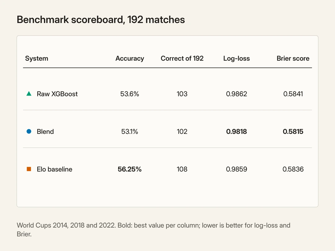
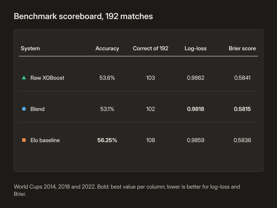
Two of those numbers deserve a definition. For a forecast that puts probability p on the outcome that actually happened, the log-loss is the mean of −ln p, and the multiclass Brier scoreBrier scoreFor each match, the squared errors of the three outcome probabilities are added up; the score is the average of that sum over all matches. Lower is better.See in the glossaryClose adds up the squared errors of the three outcome probabilities for each match and averages that sum over the matches:

Both reward a forecaster for being confident and right and punish confident and wrong; both are minimised by honest probabilities, which is why they, not accuracy, are the metrics I lean on for a probabilistic model.

The blend does not beat Elo on accuracy. The simple baseline is ahead by six matches of 192. My first instinct was disappointment. My second, better instinct was to ask the only question that matters: is a 3.1-point accuracy gap on 192 matches even real?

Because both systems are scored on the same matches, this is a paired comparison, so the right tool is McNemar's testMcNemar's testA paired test that counts only the matches where one system was right and the other wrong, and asks whether one of them came out ahead more often than chance allows.See in the glossaryClose, not a two-sample test. McNemar's test counts only the matches where one system was right and the other wrong, and asks whether one of them came out ahead more often than chance allows. Of the 192 matches, the blend and the baseline picked different outcomes in 17. In one of those (Russia against Croatia in 2018) both were wrong; in the other 16 exactly one system was right: the blend alone in 5, the baseline alone in 11, a net edge of six matches to Elo. The exact two-sided McNemar test on those 16 matches gives p = 0.21: the paired test found no statistically significant difference in accuracy.

The probabilities tell a slightly different story. A paired bootstrap (resampling the 192 matches with replacement thousands of times to see how far the result can swing) on the per-match log-loss difference (blend minus Elo) gives a point estimate of −0.004 in the blend's favour, with a 95% interval of [−0.025, +0.018] that comfortably straddles zero. In plain terms: this benchmark provides no statistically significant evidence that either system is better.

So the defensible claim is not "Elo beat my model" and not "my model beat Elo". It is: the blend was less accurate than Elo, but the difference was not statistically significant. Its pooled log-loss and Brier score were both slightly lower. The 95% bootstrap interval for the log-loss difference included zero.

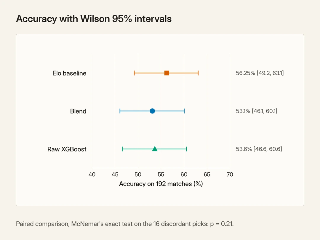
Two notes belong here. First, this is a like-for-like test: the backtested blend is the exact inference procedure the app serves, with the same symmetry-averaged probabilities, the same venue contract and the same fixed draw share, evaluated walk-forward and not a more flattering variant tuned for the write-up. Second, although the blend weight was selected only on the earlier 2006 and 2010 tournaments, I did look at the 2014, 2018 and 2022 results while iterating, so this benchmark should be read as a retrospective walk-forward evaluation rather than a never-observed final test. In the 2026 results below, the four forecasts logged before kickoff are examined separately from the 100 recomputed afterwards.

What the evaluation protocol changed

The numbers above are not the ones I first computed. My first benchmark updated each team's ratings, form and head-to-head record match by match during the tournament being evaluated, so the model predicting a quarter-final knew what had happened in the group stage. No future result leaked into training, but in-tournament form leaked into the "pre-match" features of later rounds. That is not how the live system can work: on the eve of the final its state is what it was before the opening game, plus whatever it has recorded since, and in the frozen deployment it has recorded nothing.

Correcting this (one frozen pre-tournament snapshot per tournament, the condition the deployed app actually works under) and adding the venue contract changed every number. The blend's accuracy fell from 56.25% to 53.1%; the baseline's fell from 57.8% to 56.25%. The asymmetry matters: the protocol change as a whole cost the model that uses recency features about twice as much as it cost Elo, which is what you would expect if in-tournament form is exactly what those features consume. Because the frozen state and the venue contract changed together, this comparison does not separate their two contributions. The venue contract, applied to both systems, also made the host matches harder rather than easier, since host favourites lost more often than their priors expected in these three tournaments. And the McNemar p-value moving from 0.58 to 0.21 is a protocol change, not evidence accumulating toward significance; it should not be read as a trend.

By tournament

Breaking the pooled numbers apart (64 matches each), the picture is uneven, and Elo leads accuracy in all three:

• 2014 (64)
  • Blend: Accuracy 56.3%, Log-loss 0.9559, Brier 0.5688
  • Elo baseline: Accuracy 59.4%, Log-loss 0.9651, Brier 0.5750
  • Raw XGBoost: Accuracy 56.3%, Log-loss 0.9572, Brier 0.5695
• 2018 (64)
  • Blend: Accuracy 53.1%, Log-loss 0.9575, Brier 0.5656
  • Elo baseline: Accuracy 56.3%, Log-loss 0.9510, Brier 0.5625
  • Raw XGBoost: Accuracy 53.1%, Log-loss 0.9674, Brier 0.5707
• 2022 (64)
  • Blend: Accuracy 50.0%, Log-loss 1.0320, Brier 0.6102
  • Elo baseline: Accuracy 53.1%, Log-loss 1.0416, Brier 0.6133
  • Raw XGBoost: Accuracy 51.6%, Log-loss 1.0340, Brier 0.6121

Per-tournament breakdown. The blend's lower log-loss and Brier come in 2014 and 2022; in 2018 Elo is better on all three metrics. The match-weighted averages of these rows reconcile to the pooled numbers in Figure 3.

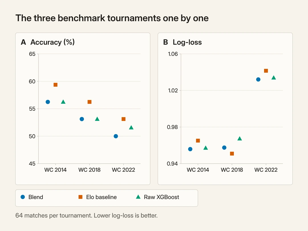
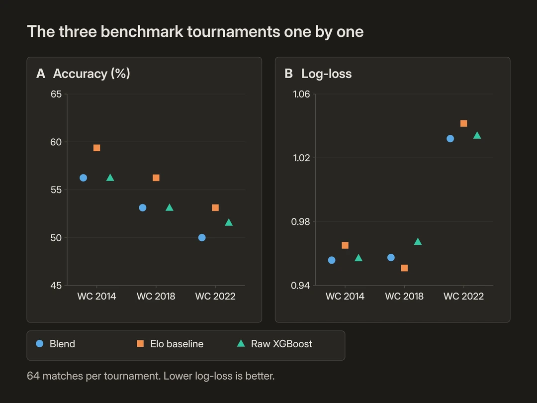
So the probabilistic story reads: the blend's lower pooled log-loss and Brier are real arithmetic, but they rest on two of three tournaments and the interval on the log-loss difference includes zero, so I will not sell them as a dependable advantage. They are also scores of overall forecast quality, not a calibrationCalibrationWhether stated probabilities match reality: outcomes given 60% should happen about 60% of the time. The expected calibration error (ECE) measures the gap.See in the glossaryClose verdict on their own. A cross-system calibration check (calibration asks whether outcomes given 60% really happen about 60% of the time; here the expected calibration error on the top-class confidence, 10 equal-width bins) ranks the three the same way: blend 0.040, raw XGBoost 0.047, Elo 0.054, all small on 192 matches.

One more number. The benchmark contains 41 draws, and none of the three systems called any of them. The blend and Elo never picked a draw in the 192 matches; raw XGBoost picked a draw once (Russia against Uruguay in 2018), and that match was not a draw. This is about the most likely outcome, not about draw probability, which every system still assigns. No system here meaningfully predicts draws; the draw class is the known pathology of three-way football models, and it is now on the record rather than hidden in an average.

To anchor the metrics: three-class log-loss for random guessing is ln 3 ≈ 1.099; both the blend (0.982) and Elo (0.986) clear that, but only modestly. A uniform Brier score is 0.667; 0.58 is comfortably better than random. Both systems are genuinely informative, and they land in almost the same place. That near-tie is the thesis of the project: on this retrospective World Cup benchmark, nothing I built extracted meaningfully more than a simple Elo rating from my public-data feature set. This echoes the academic finding (Lasek et al., 2013; Hvattum and Arntzen, 2010) that Elo systems are remarkably strong baselines for football. I would stop short of calling this a ceiling for all football data; 192 matches cannot support that. But for the data and features I had, Elo was the thing to beat, and the best I managed was no detectable difference on picks, with slightly better probability scores.

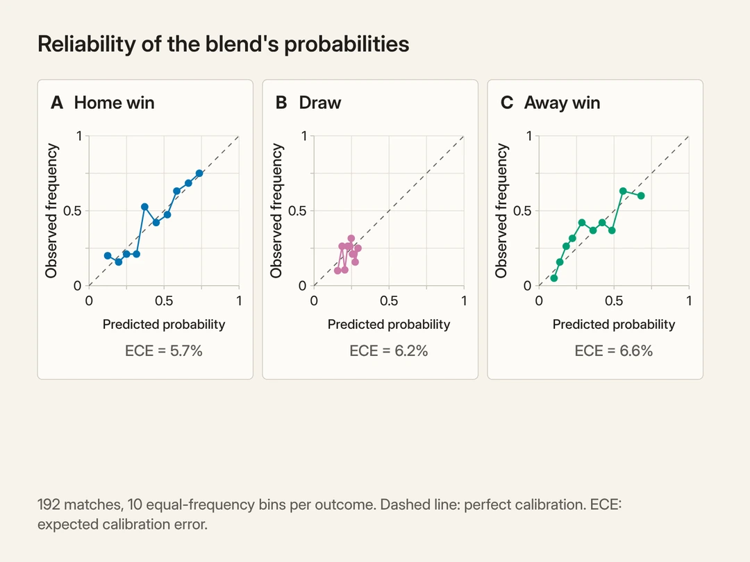
Every number in this section is reproducible. The row-level backtest predictions, the per-tournament and pooled summaries, the paired tests, the protocol comparison, the figures and the data checksums are tracked in the repository's reports/ directory.

Scorelines: a Dixon and Coles layer that cannot contradict itself

The headline model only outputs win, draw and loss. People also want a scoreline, so I added one, carefully. The classic approach models each side's goals as a Poisson count (the textbook distribution for events that occur at a steady average rate; Maher, 1982), refined by Dixon and ColesDixon and Coles modelA scoreline model that treats each side's goals as a Poisson count and corrects the four low-scoring results (0-0, 1-0, 0-1 and 1-1), where goals are not independent.See in the glossaryClose (1997) with a correction for the dependence in low-scoring games. The probability of i home goals to j away is

where the Poisson terms model each side's goals and the correction τ, with its parameter ρ, nudges the four lowest scorelines (0-0, 1-0, 0-1 and 1-1) toward how real low-scoring matches behave.

My twist is a consistency constraint. Rather than fit an independent scoreline model that might disagree with the probabilities already on screen, I solve for the expected-goals pair (λ_home, λ_away) whose Dixon and Coles grid rolls back up to the win, draw and loss probabilities being shown, within a small numerical tolerance (the smoke test holds the roll-up to within 1.5 percentage points). The most likely scorelines are then read off that grid. Consistency with the headline numbers is enforced, not left to chance.

One disclosure: ρ is fitted once by maximum likelihood on the frozen history (−0.0500 on 49,404 matches) and used as the constant −0.05. Because the scoreline layer is presentation only and is never scored in any evaluation, this introduces no leakage into any reported metric.

What the SHAP explanation covers

A probability with no reason behind it is hard to trust, so each prediction comes with a plain-language explanation built on SHAPSHAPA method that divides one prediction into the contribution of each input feature. Here it shows which factors raised or lowered the first team's raw win score in XGBoost.See in the glossaryClose (Lundberg and Lee, 2017), a method that divides a prediction into the contribution of each input feature, computed here with the exact TreeSHAP algorithm for tree ensembles (Lundberg et al., 2020).

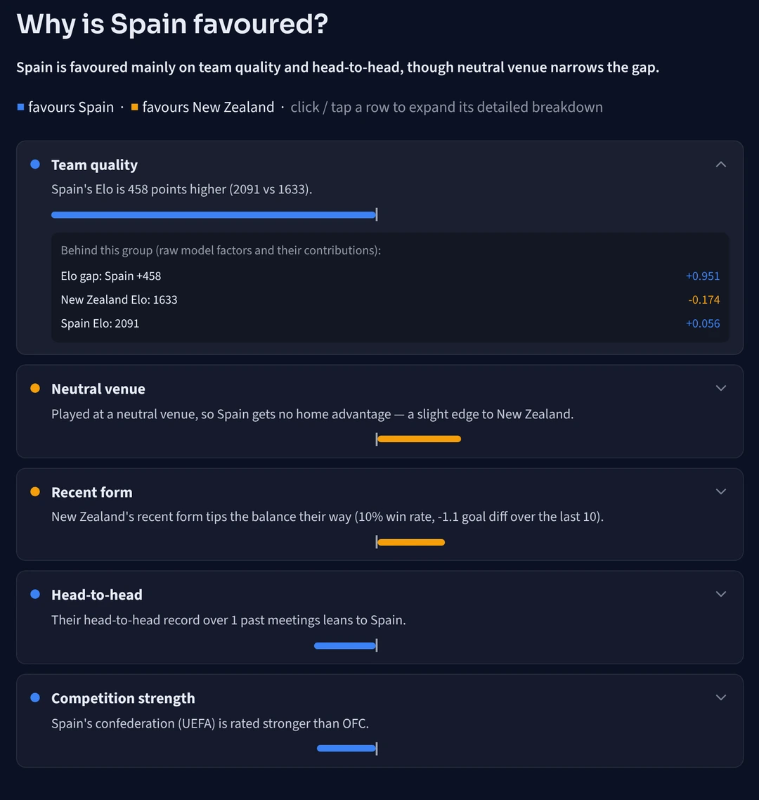
SHAP attributes a model's output additively across its features, but 31 features, several of them one-hot confederation flags, make for a noisy explanation. So I sum the SHAP values into a fixed handful of human-readable buckets: team quality, recent form, competition strength, head-to-head and neutral venue. Because SHAP is additive, the grouped sums reconcile exactly to what they explain; a smoke test asserts this to within 10⁻⁴ on every check.

One clarification. SHAP here explains the raw XGBoost component, not the final card probability, and it is additive in margin (logit) space, not probability space: for each class, the base value plus the summed contributions equals that class's raw margin, and a softmax turns the three margins into probabilities. The final number is then formed by shrinking those probabilities a quarter of the way toward the Elo prior. Read the panel as the model-derived evidence behind the prediction, why the learner leans the way it does, rather than a full decomposition of the blended probability. The explanation is oriented to the first team's win, so in a close match "lowers the margin" does not cleanly map to "favours the other team"; it can favour the draw instead. A rigorous multiclass attribution would contrast the favoured and runner-up margins, and that is on the future-work list.

From one match to a tournament: Monte Carlo

A match model becomes a tournament model by Monte Carlo simulationMonte Carlo simulationPlaying the whole tournament thousands of times, with each match drawn at random from the model's probabilities, and counting how often each team reaches each stage.See in the glossaryClose, which means playing the whole tournament many times with the randomness drawn from the model's probabilities. I play the entire 2026 bracket, 12 groups of four and then the full knockout ladder from the round of 32 (where the eight best third-placed teams join the group winners and runners-up) down to the final, thousands of times, sampling each match from the model's probabilities and tracking how often each team reaches each stage and lifts the trophy. Within a group I rank teams on points, then overall goal difference, then goals scored, then the head-to-head record among level teams; anything still tied is settled randomly. That order is my simplification, not the regulations': the official 2026 rules separate teams level on points by their head-to-head results first, and only then by overall goal difference, goals scored, fair play and FIFA ranking. The criteria I model decide the vast majority of groups, but the ranking method inside a group should be read as simplified. The allocation of third-placed teams, by contrast, is taken from the regulations exactly. Knockout draws go to a probability-weighted shootout.

The fiddly part of a 48-team bracket is the round of 32. Which third-placed group feeds which slot is fixed by a published combination table (Annexe C of the FIFA 2026 regulations), one assignment for each of the C(12, 8) = 495 ways the eight qualifiers can fall. The simulator implements that table directly and validates all 495 rows at load time, as a bijection (every qualifying third placed exactly once) and against the bracket's eligibility constraints (no team lands in a disallowed slot or replays a group opponent), so the bracket geography is officially correct, not merely plausible.

Because the simulator consumes probabilities, not hard picks, calibration pays off directly: better match probabilities mean more trustworthy bracket odds.

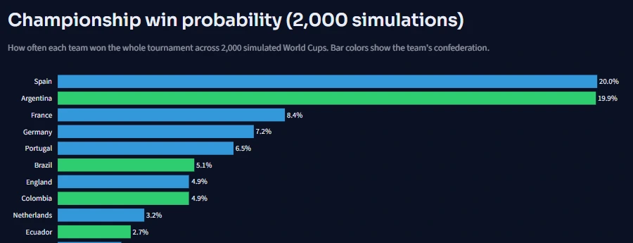
Two other versions of this outlook exist. The audited simulator described in the next section, run with the same seed (the starting value that fixes the sequence of random draws), puts Argentina narrowly ahead, 20.1% against Spain's 18.6%. And one public record exists from before the tournament: a LinkedIn post (opens in a new tab) published on 11 June 2026 at 13:55 UTC, before the opening match kicked off, carried the simulator's championship outlook as it then stood (10,000 runs, before the audit): Spain 20.9%, Argentina 18.1%, France 8.2%, Brazil 7.8%. It is a public timestamp, not a scored forecast, and it is not part of the evaluation.

How the app serves predictions, and what the audit found

A model that only runs on my laptop is not a project, so the system is built like a small service: a four-page app (Match Predictor, Prediction Tracker, Tournament Simulator and Team Rankings) deployed to a public host.

The piece I care most about is the Prediction Tracker, and it is also where the audit before publication found the most important problem. The intended guarantee was simple: every prediction for a 2026 match comes from a model and a team-state snapshot whose data ends before the tournament began, so the model has never seen a World Cup 2026 result. The cutoff is drawn at the tournament, not the calendar year: training includes every international up to the eve of the opening match, with the last match on 10 June 2026, and excludes only the World Cup fixtures being predicted. One dating fact belongs here: the model file evaluated in this article was built on 13 July 2026, during the tournament, from that frozen data; its manifest records the build time and the checksums. So what this article can support is a claim about the data cutoff, not that this exact file existed before the opening match. Live scores arrive from a football results API and are compared against those forecasts.

What the audit found is that the deployed app did not honour that guarantee strictly. Each time it restarted after a period of inactivity, it downloaded the current dataset and retrained a model, so during the tournament the public app was serving a model trained on a slightly different snapshot (one extra row and a different early-stopping point) from the one evaluated here. No World Cup 2026 result ever entered its training data, so the temporal guarantee held, but "the same model" did not. The fix is in place: the frozen model and its serving data are now tracked in the repository with their checksums, the app loads them instead of retraining, and it refuses to serve anything if a checksum does not match the manifest.

The second lesson concerns pre-registration. Forecasts regenerated on the fly from frozen inputs are leakage-free, but they are not evidence that a specific number was published before a specific match. For the last four matches of the tournament I therefore wrote an append-only prediction ledger: each row records both systems' probabilities, the venue, the model's checksum, the code commit and the time of generation, with a flag that the row was written before kickoff. The semi-finals were logged on 13 July, the third-place match and the final on 16 July. The ledger has never been edited, and the evaluation reads it, not the app. Its limit: each row records when it was generated, in UTC, but not the official kickoff time, so the "before kickoff" check compares dates, not hours.

Holding it all together is a pre-push smoke test: it loads the frozen bundle and its serving state (a separate test asserts their checksums against the manifest), verifies that predictions are valid probabilities, checks the symmetry of neutral predictions, confirms the scoreline grid rolls up within tolerance, checks the SHAP reconciliation, validates the round-of-32 table and runs a small Monte Carlo. A git hook blocks any push that fails it, and it has caught real regressions.

Results at the 2026 World Cup

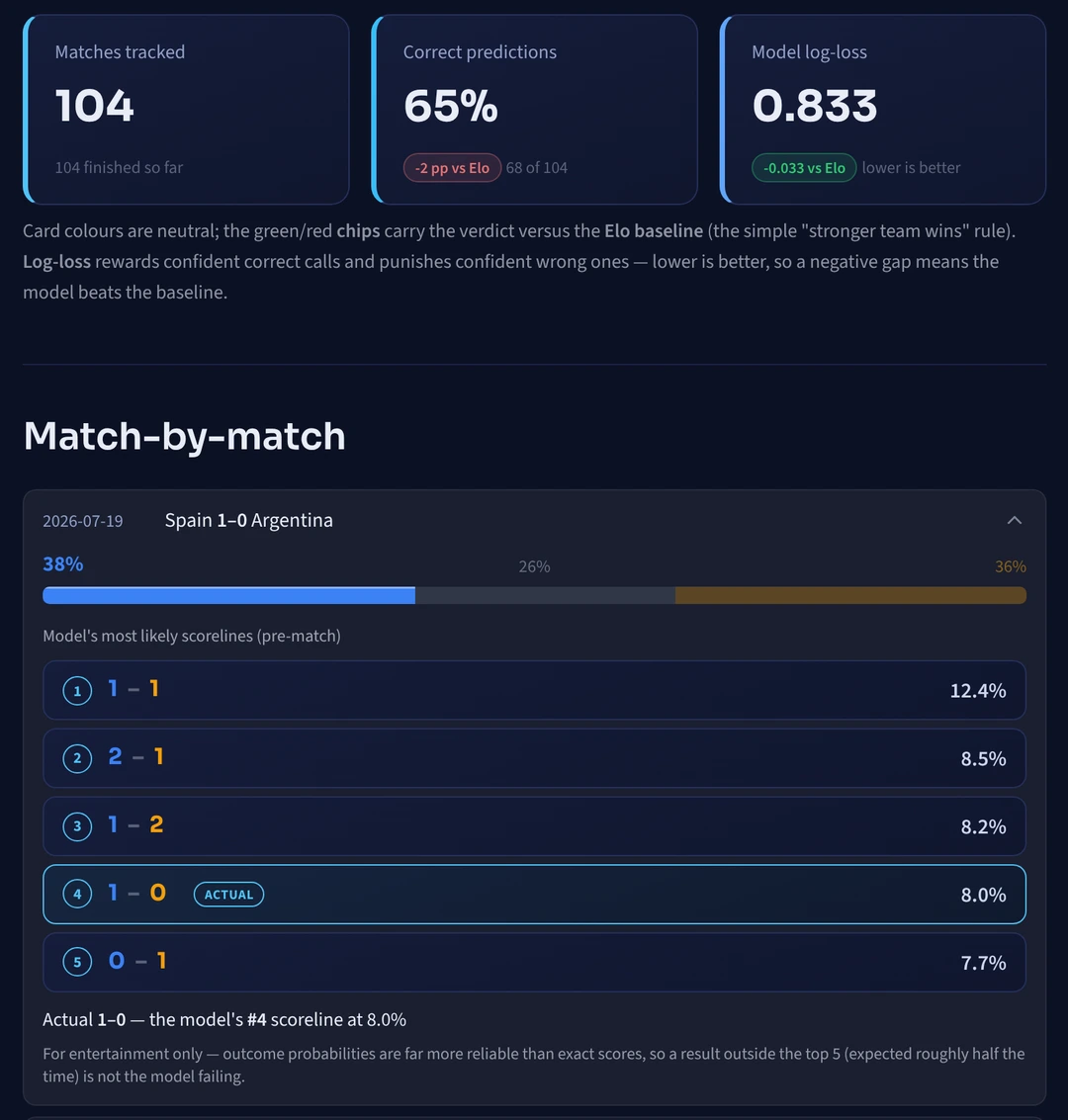
The tournament ran from 11 June to 19 July 2026. Spain beat Argentina 1-0 after extra time in the final; England beat France 6-4 in the third-place match. All 104 matches were scored under the training convention (after extra time, shootouts as draws): 95 ended in regular time, 5 in extra time and 4 on penalties.

The forecasts fall into two groups, and they should not be mixed.

The four forecasts logged before kickoff

The four ledger rows are the only match forecasts that can be called pre-registered. The blend favoured Spain over France, Argentina over England, France over England and Spain over Argentina. Three of the four came true; England's 6-4 win over France was the miss. Elo favoured the same four teams, so on picks the two systems are identical here. On the four matches the blend's log-loss was 0.892 and Elo's 0.870; with four observations no test is meaningful, and I report the numbers only for completeness.

The 100 forecasts recomputed afterwards

The other 100 forecasts are produced by the same frozen model and frozen state, but they were computed after the fact, when I ran the full evaluation. They are out of sample in the strict sense (no result from the 2026 World Cup entered training; internationals up to 10 June 2026 did), but they are not pre-registered, and a reader is entitled to weigh them accordingly. On these 100 the blend got 65 right and Elo 67.

All 104 matches

The blend was right on 68 of 104 (65.4%) and Elo on 70 of 104 (67.3%). The two systems disagreed on only two matches, and Elo was right both times; McNemar's test gives p = 0.50. On probabilities the picture is clearer than on the benchmark: the blend's log-loss was 0.833 against Elo's 0.867, Brier 0.487 against 0.507, and the paired bootstrap interval on the per-match log-loss difference is [−0.059, −0.005], excluding zero. On the 100 recomputed matches alone the interval is [−0.063, −0.007].

So did the retrospective finding hold up live? In its most important part, yes: the blend did not pick winners better than a plain Elo rating. Both systems were more accurate at this tournament than on the benchmark (about 65% against 53 to 56%), which says something about the 2026 draw rather than about the models; favourites won more often. Where the live result differs is on probability quality. The blend's edge on log-loss, which the benchmark could not separate from zero, came out larger here and with an interval that excludes zero. I take that as encouraging, not conclusive: it is one tournament, and 100 of its 104 forecasts were recomputed rather than pre-registered. What the comparison shows is the observation itself: on these 104 matches the blend had a lower log-loss than Elo, with almost the same picks. The model section suggested that shrinking XGBoost toward the Elo prior would improve the probabilities, but this comparison, blend against Elo, cannot isolate that cause.

Limitations and what I would do next

I have flagged the weaknesses throughout; here they are in one place, roughly in the order I would tackle them.

• A learned draw model. My hypothesis, with no ablation isolating it, is that the fixed 0.227 draw rate costs the blend performance, and the zero draw picks in the evaluation are its symptom. Letting draw probability vary with the strength gap, as the Poisson and Dixon and Coles family does naturally, is the first experiment I would run.
• A competition-aware Elo. A constant K = 40 ignores that a World Cup match should move ratings more than a friendly. A margin-aware, importance-weighted K would make the baseline itself stronger and fairer.
• A bigger evaluation. 192 benchmark matches cannot resolve a two- or three-point edge, and 104 live matches are one tournament. A rolling-origin holdout across all internationals would add statistical power.
• Pre-registration from the first match. The ledger should have started on 11 June and recorded both the time of each forecast and the official kickoff time, not started on 13 July without kickoff times.
• Richer features. Player-level data (squad quality, key absences) and opponent-adjusted form are the obvious sources of signal the current public-data model cannot see.

The main finding, in one sentence:

On a 192-match retrospective World Cup benchmark and on the 104 matches of the 2026 World Cup, the XGBoost and Elo blend did not pick winners better than a plain Elo rating, and the paired tests found no significant accuracy difference in either case. Its probabilities were somewhat better: numerically on the benchmark, where the bootstrap interval included zero, and more clearly at the 2026 World Cup, where it did not.

That is not the clean win I wanted when I started. What it showed me is this: at the World Cup, on public data, the higher-rated team usually wins; a richer model mostly rediscovers that fact and, at best, gives somewhat better probabilities; and a good model should say so while being clear about how often it will be wrong.

Code and data

Source code, evaluation reports, the frozen model and serving data with their checksums, the prediction ledger, the row-level backtest and live predictions and the generated figures are in the public repository (opens in a new tab). The research app (opens in a new tab) serves that frozen model; its first start after a period of inactivity may take a few minutes. The short version of this work is on its Project page.

Glossary

Elo rating

A strength score for each team, borrowed from chess. Every team starts at 1500; after each match, a team's rating changes by the gap between the actual result and the expected one, so even a draw can move it.

XGBoost

A machine-learning method that grows hundreds of small decision trees in sequence, each one correcting the mistakes of the trees before it.

Elo prior

An estimate of the win, draw and loss probabilities from the two teams' Elo ratings. In this project it carries 25% of the final prediction.

Blend

The model that combines, for each outcome, the XGBoost probability with weight 75% and the Elo prior with weight 25%. The app shows its probabilities.

Calibration

Whether stated probabilities match reality: outcomes given 60% should happen about 60% of the time. The expected calibration error (ECE) measures the gap.

Log-loss

A score for probability forecasts that rewards confident correct calls and punishes confident wrong ones. Lower is better.

Brier score

For each match, the squared errors of the three outcome probabilities are added up; the score is the average of that sum over all matches. Lower is better.

Walk-forward backtest

Train only on matches before a tournament, test on that tournament, step forward in time and repeat. It imitates forecasting as it would have happened.

Confidence interval

A range that shows the uncertainty of an estimate. Here, when the interval for the difference between two models includes zero, the data are also consistent with no difference.

Wilson interval

The range of true accuracies that is consistent with a count of correct picks, here at 95% confidence.

McNemar's test

A paired test that counts only the matches where one system was right and the other wrong, and asks whether one of them came out ahead more often than chance allows.

p-value

If the two systems were truly equally accurate, the probability of seeing a difference at least this large in the test. Here it comes from McNemar's test.

Paired bootstrap

Resampling the same matches with replacement thousands of times, so that a match can appear more than once in a sample, and comparing both models on each resample to see how far the difference between their scores could swing. In this article it gives the intervals for the log-loss difference between the two models.

Dixon and Coles model

A scoreline model that treats each side's goals as a Poisson count and corrects the four low-scoring results (0-0, 1-0, 0-1 and 1-1), where goals are not independent.

SHAP

A method that divides one prediction into the contribution of each input feature. Here it shows which factors raised or lowered the first team's raw win score in XGBoost.

Monte Carlo simulation

Playing the whole tournament thousands of times, with each match drawn at random from the model's probabilities, and counting how often each team reaches each stage.

References

1. Brier, G. W. (1950). Verification of forecasts expressed in terms of probability (opens in a new tab). Monthly Weather Review, 78(1), 1–3.
2. Brown, L. D., Cai, T. T., and DasGupta, A. (2001). Interval estimation for a binomial proportion (opens in a new tab). Statistical Science, 16(2), 101–133.
3. Chen, T., and Guestrin, C. (2016). XGBoost: A scalable tree boosting system (opens in a new tab). In Proceedings of the 22nd ACM SIGKDD (pp. 785–794).
4. Dixon, M. J., and Coles, S. G. (1997). Modelling association football scores and inefficiencies in the football betting market (opens in a new tab). Journal of the Royal Statistical Society: Series C, 46(2), 265–280.
5. Elo, A. E. (1978). The Rating of Chessplayers, Past and Present. Arco Publishing.
6. Fédération Internationale de Football Association. (2026). Regulations: FIFA World Cup 26 (11 June to 19 July 2026) (opens in a new tab), including Annexe C, the round-of-32 combination table. FIFA.
7. Forrest, D., Goddard, J., and Simmons, R. (2005). Odds-setters as forecasters: The case of English football (opens in a new tab). International Journal of Forecasting, 21(3), 551–564.
8. Gneiting, T., and Raftery, A. E. (2007). Strictly proper scoring rules, prediction, and estimation (opens in a new tab). Journal of the American Statistical Association, 102(477), 359–378.
9. Goddard, J., and Asimakopoulos, I. (2004). Forecasting football results and the efficiency of fixed-odds betting (opens in a new tab). Journal of Forecasting, 23(1), 51–66.
10. Hvattum, L. M., and Arntzen, H. (2010). Using ELO ratings for match result prediction in association football (opens in a new tab). International Journal of Forecasting, 26(3), 460–470.
11. Jürisoo, M. International football results from 1872 to present (opens in a new tab) [Data set]. GitHub. (snapshot frozen for this project with its last match on 10 June 2026; the checksums of the raw file, the processed history and the trained model are recorded in models/model-manifest.json in the project repository).
12. Lasek, J., Szlávik, Z., and Bhulai, S. (2013). The predictive power of ranking systems in association football (opens in a new tab). International Journal of Applied Pattern Recognition, 1(1), 27–46.
13. Lundberg, S. M., and Lee, S.-I. (2017). A unified approach to interpreting model predictions (opens in a new tab). NeurIPS 30. arXiv:1705.07874
14. Lundberg, S. M., et al. (2020). From local explanations to global understanding with explainable AI for trees (opens in a new tab). Nature Machine Intelligence, 2(1), 56–67.
15. Maher, M. J. (1982). Modelling association football scores (opens in a new tab). Statistica Neerlandica, 36(3), 109–118.
16. Niculescu-Mizil, A., and Caruana, R. (2005). Predicting good probabilities with supervised learning (opens in a new tab). In Proceedings of the 22nd ICML (pp. 625–632).
17. World Football Elo Ratings, methodology (opens in a new tab).

Tournament format and the round-of-32 combination table (Annexe C) follow the official competition regulations (FIFA, 2026); the in-group ranking used by the simulator is a disclosed simplification (see the Monte Carlo section).

Note on tooling: the analysis, modelling, code, evaluation and conclusions in this article are my own. I used an AI coding assistant to help structure and copy-edit the prose; every word carried my final approval.